Predicting Hard Drive Failure with Machine Learning

One of the top applications of artificial intelligence and machine learning is predictive maintenance - Forecasting the probability of machinery breaking down in order to perform service before the damage is done.

A case for predictive maintenance

Equipment downtime is very costly to a manufacturer, since it might delay an entire factory line which is dependent on a process being performed by one of the machines in the line. On the other hand, unnecessarily servicing machines is also quite costly, as we might be paying someone to go waste their time inspecting machines which are in perfect order.

With historic data collected for a number of machines, we can use machine learning to predict the probability of breakdown for a piece of equipment within a window of time in the future, such as within the next seven days.

Many industrial machines are now becoming IoT-enabled, where each machine is equipped with sensors and logging capabilities which can be streamed to a central hub for analysis. This enables powerful use of machine learning algorithms.

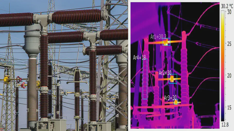
As an example, it has been found possible to perform early fault detection in Chinese power substations with more than 80% accuracy using thermal imagery and deep learning [1]. Another example comes from Siemens Corporation, where a ROC AUC score of 0.7 was achieved using logs from specific components in medical equipment [2].

What you need

In order to build machine learning models for predictive maintenance, you need data. Ideally, you’ll want a couple of years worth of historic data for a broad distribution of machines which are of the same type. It is also important, that failures of these machines are stored and annotated in your dataset.

There are several sources of data which can be considered:

• Internal sensor data, such as temperature, sound, light, etc.
• External sensor data, such as thermal imagery.
• Machine logs, such as logged errors and events.

These approaches can be applied both on the machine-level or the component-level, depending on the desired specificity of the model.

A representation problem

When developing machine learning models you’ll often want each class in the dataset to be evenly represented to avoid introducing bias.

If 99% of your dataset represents a single class, it is highly likely that a machine learning algorithm will simply learn to always predict this class when prompted - After all, it would be correct in 99% of all cases.

One of the big challenges when doing predictive maintenance with AI is the fact that equipment failures are usually underrepresented in the dataset. This is because machines usually run as they should: Failure is an anomaly. If your machines are broken half of their lifetime, you will have other problems to consider before diving into predictive maintenance.

Therefore, we need to be careful to prepare our data and select our algorithms so that we deal with this issue. Some ways of addressing this problem are:

• Undersampling our data so that classes are more evenly represented.
• Augmenting underrepresented classes to synthetically produce more training examples.
• Using certain algorithms that are less sensitive to class imbalance such as Support Vector Machines.

BackBlaze hard drive data

As a practical example of how we can approach predictive maintenance using sensor data, we will predict the likelihood of hard drive failure using S.M.A.R.T. sensor data.

Each quarter, the online backup company BackBlaze provides a daily event log for each of their hard drives, detailing its model, serial number, S.M.A.R.T. parameters and whether it has failed that day. Just what we need!

Here are some example rows from the BackBlaze dataset:

As you can see, we have model, serial number, failure and a number of S.M.A.R.T. parameters represented (both raw and normalized values). The availability of these parameters can depend on the specific vendor and model of hard drive - Therefore, we will see missing values in some S.M.A.R.T. parameter columns where the hard drive vendor did not supply them.

For this experiment, I have compiled BackBlaze’s data for the last 2 years and dropped columns which are raw, static or have more than 30% missing values. Additionally, I have filled remaining missing values with their column’s most frequent value (their model).

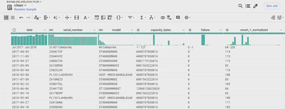
In order to effectively prepare and clean big datasets, I can recommend the Dataprep tool on Google Cloud Platform. Dataprep enables you to make “recipes” for transformations on a sample of your dataset and then apply those transformations on the entirety of your dataset in parallel with a Dataflow job. Very handy!

After the data has been prepared and cleaned, it is stored in a Google Cloud BigQuery database, so we can access it efficiently later.

“Bagging” the data

Now, for each failed hard drive, we want to get events prior to the failure and perform calculations on them in order to make a dataset of time series to analyze. We will use three windows of time:

• Historical context: 7 days
  This marks the amount of time to look back for historical information on the basis of which to make a prediction.
• Prediction window: 7 days
  This is the amount of time before a failure we want to be able to predict.
• “Infected” window: 14 days
  This amount of time after a failure, we assume that the data does not represent the normal operation of a hard drive and therefore we will not use it for “healthy” hard drive examples.

We will take each logged hard drive failure and make a bag for each 7 days (prediction window) that came before it which contains all events 7 days prior to it (historical context).

This will leave us with 7 “event bags”, each of which containing a 7 day historical context. In this historical context, there will be a number of S.M.A.R.T. parameters for each day. We can do some calculations on these parameters, such as the percentage difference in one parameter since yesterday, 1 days, 3 days, 5 days, etc.

We mark these 7 bags with “failure”, as we know the hard drive fails within these 7 bags. The new dataset will look something like this:

Finally, we perform the same procedure for healthy intervals - These are taken from intervals which are not in the prediction window or the infected window.

Now we have a lot of nice, flat, new data for “healthy” and “infected” hard drive intervals, and we need not keep the time series data around anymore. I have chosen to undersample the healthy hard drive data, making a dataset of approximately 20.000 examples, where 10.000 of those examples are failed hard drive event intervals.

Classifier algorithm

With a dataset in place, we are ready to create our classifier! First, we shuffle the dataset and split it into training and validation sets using a 75/25 split.

It turns out, that simple single-layer self-normalizing neural network performs very well for this problem. Using Keras, we can define a function to prepare such a network:

 1
 2
 3
 4
 5
 6
 7
 8
 9
10
11
12
13
14
15
16
17
18
19
20
21
22
23
24
25
26
27
28
29
30
31
32
33
34
35
36

from keras.models import Sequential
from keras.layers import Dense, AlphaDropout

def prepare_dnn_binary_classifier(input_dim, 
                                  num_layers, 
                                  diminish_factor, 
                                  use_dropout=False, 
                                  dropout_factor=0.3, 
                                  optimizer = "rmsprop"):
    model = Sequential()
    model.add(Dense(input_dim, 
                    input_dim=input_dim, 
                    activation="selu", 
                    kernel_initializer='lecun_normal'))

    if use_dropout:
            model.add(AlphaDropout(dropout_factor))

    carried_size = input_dim

    for layer in range(num_layers - 1):
        carried_size = int(max(carried_size / diminish_factor, 1))
        model.add(Dense(carried_size, 
                        activation="selu", 
                        kernel_initializer='lecun_normal'))

        if use_dropout:
            model.add(AlphaDropout(dropout_factor))

    model.add(Dense(1, activation="sigmoid"))

    model.compile(optimizer=optimizer, 
                  loss='binary_crossentropy', 
                  metrics=['accuracy'])

    return model

To instantiate, fit and evaluate the model, we do:

 1
 2
 3
 4
 5
 6
 7
 8
 9
10
11
12
13

import sklearn.metrics as metrics

model = prepare_dnn_binary_classifier(dim, 1, 2, use_dropout=True)
model.fit(train_x, 
          train_y, 
          epochs=5, 
          validation_data=[test_x, test_y])

preds_y = model.predict(test_x)

print("F1 score: %f" % metrics.f1_score(test_y, np.round(preds_y)))
print("ROC AUC score: %f" % metrics.roc_auc_score(test_y, preds_y))
print(metrics.confusion_matrix(test_y, np.round(preds_y)))

After fitting this model, we get an impressive ROC AUC score of 0.98 and the confusion matrix reveals very few false positives and false negatives.

However, such a good score could be cause for concern - It is very possible that the dataset is not big enough and the model might not generalize perfectly to new events.

But it does indicate the potential effectiveness of predicting hard drive failure this way, even though the precision can be expected lower when applied to a bigger dataset.

Additionally, we can apply a Support Vector Machine to this same dataset for validation and to gain more insight:

1
2
3
4
5
6
7
8
9

from sklearn.svm import LinearSVC

svm_model = LinearSVC()
svm_model.fit(train_x, train_y)
preds_y_svm = svm_model.predict(test_x)

print("F1 score: %f" % metrics.f1_score(test_y, np.round(preds_y_svm)))
print("ROC AUC score: %f" % metrics.roc_auc_score(test_y, preds_y_svm))
print(metrics.confusion_matrix(test_y, np.round(preds_y_svm)))

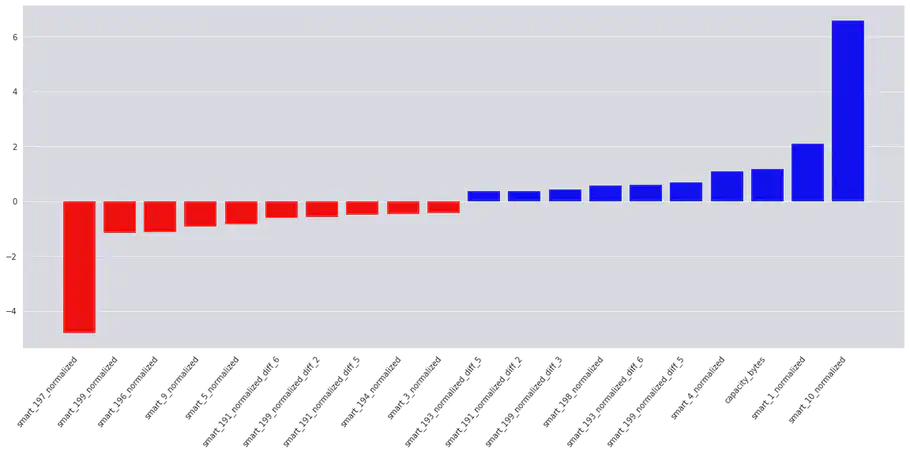
Fitting the SVM yields a similarly promising ROC AUC score of 0.98. By plotting feature importance, we get an intuition of which parameters have the biggest influence on deciding whether a drive is going to fail or not.

Interestingly, we see that momentary values of these S.M.A.R.T. parameters are important to the model:

• 199: UltraDMA CRC Error Count
• 193: Load Cycle Count
• 191: G-sense Error Rate

Due to the large amount of parameters, I have included only the 20 most important features:

Conclusion

That’s it for now! We talked about predictive maintenance, processed BackBlaze hard drive data with Google Cloud Dataprep, applied classifier algorithms using Keras, Tensorflow and Scikit-Learn and got interesting results.

However, for more reliable results, a bigger dataset should be used. This could either be done by using a bigger timeframe or a larger amount of healthy hard drive events in combination with bias insensitive classification algorithms such as Support Vector Machines.

// Maria Hvid, Machine Learning Engineer @ neurospace

References

[1] Ullah, I., Yang, F., Khan, R., Liu, L., Yang, H., Gao, B. and Sun, K., 2017. Predictive Maintenance of Power Substation Equipment by Infrared Thermography Using a Machine-Learning Approach. Energies, 10(12), p.1987.

[2] Sipos, R., Fradkin, D., Moerchen, F. and Wang, Z., 2014, August. Log-based predictive maintenance. In Proceedings of the 20th ACM SIGKDD international conference on knowledge discovery and data mining (pp. 1867-1876). ACM.