Which model performs best on detecting the quality of red wine; Artificial Neural Network or Support Vector Machine?

When dealing with a problem you must determine what model to use for solving it. You can choose between two approaches: statistics, and machine learning. If statistics cannot solve the problem, it is time to experiment with machine learning and figure out what model to use. Today, an increased focus is on the usage of artificial neural networks, which is a strong architecture for solving complex problems. However, do not forget, that in machine learning other strong algorithms exist, such as decision trees, random forests, and support vector machines. The following case is a showdown between the power of artificial neural networks and support vector machines, when determining the quality of red wine.
This dataset is interesting because it requires you go through outlier detection, correlation tests, an imbalanced dataset, missing information, and finally, we can detect how well two strong algorithms perform on the same terms.
Introduction to the dataset
The dataset provided is from Kaggle. The data is retrieved by five wine experts P. Cortez, A Cerdeira, F. Almeida, T. Matos, and J. Reis. All wine tasted is from the same province in Portugal, and consist of a total of 1599 red wines and 4898 white wines. Each wine has been evaluated through a score between zero (very bad) to ten (very good) [1].
The dataset contains 11 input features:
- Fixed acidity
- Volatile acid
- Citric acid
- Residual sugar
- Chlorides
- Free sulfur dioxide
- Total sulfur dioxide
- Density
- pH
- Sulphates
- Alcohol and one output variable: Quality
Due to privacy and logistic issues, the dataset do not inform about the type of wine grape, sales price, or wine brand. Additionally, no information is given to how the five authors determine the score (anonymously, average of total score etc).
Explore the dataset of red wine
The dataset has no missing values, and is in the exploring phase split in to red wine and white wine because we have a hypothesis that the feature importance is different in red wine and white wine.
For this showdown, we will only be looking at red wine. To get an understanding of the distribution, we can look at how many observations are presented on each quality level (0 - 10):
|
|
| Quality value | 3 | 4 | 5 | 6 | 7 | 8 |
|---|---|---|---|---|---|---|
| n | 10 | 53 | 681 | 638 | 199 | 18 |
| percentage | 0.63% | 3.31% | 42.59% | 39.90% | 12.45% | 1.13% |
From this, it can be concluded that the dataset is highly imbalanced. Not only is the majority of the red wines classified as a quality level of 5 or 6, there also do not exist any observations on each end of the scale, making it hard for our model to learn about these five scores (0 to 2, and 9 to 10).
Correlation and HeatMap
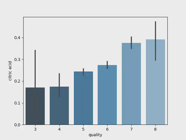
To see whether there exist a visual linear correlation between the input features and the output variable we can use bar plots. We will use seaborn for creating these plots with just few lines of code:
|
|

Barplot for citric acid
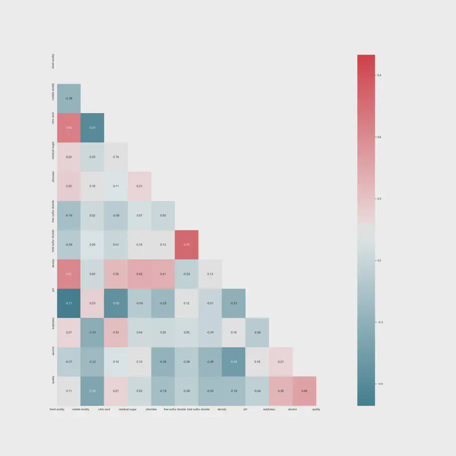
Even though the bar plot indicates a linear relationship, it is difficult to be certain because the confidence interval shows an uncertainty. Therefore, a Spearman correlation test is made to get an understanding of the power of the correlations. First we use a heatmap with the p-value determined by following code:
|
|
The decision rule is, that if the p-value is below 0.05, the null hypothesis of rho = 0 is rejected, and the correlation is significant. Through this test, it is determined that volatile acidity do not provide any significant impact on the model, whereas it is removed. Additionally, alcohol seems to be the most important feature to the output variable with a positive linear correlation of 0.48 and density is positively linear correlated with the amount of residual sugar (0.42), chlorides (0.41), citric acid (0.35), and fixed acidity (0.62). Additionally, the pH value has a negative linear relationship with the amount of fixed acidity (-0.71), citric acid (-0.55), and chlorides (-0.23). However, none of the input features are strong positive or negative correlated with the output variable.

HeatMap with Spearman correlation
Outlier detection
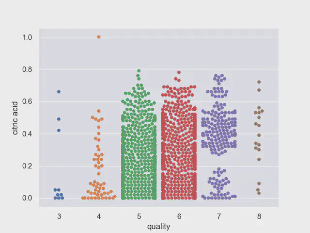
The bar plots earlier indicates, that there exist a high standard deviation in both ends of the scale. Each input features mean and standard deviation are calculated, confirming this. We can use Swarm plots to see these outliers.
|
|

Swarmplot for citric acid
In general in all swarmplots, almost all classes except where quality is 5 and 6, indicates that there are some outliers. One issue with the quality level of 3 and 8, is the small amount of representatives, making it hard to find a pattern.
The outliers detected can either be removed manually or by statistical tests which removes these automatically. We have used Tukey’s test for automatically detect and remove outliers, removing 255 observations providing the new sample size to be equal to 1,343.
This makes our improved dataset look like this:
| Quality Group | Representatives |
|---|---|
| 3 | 4 |
| 4 | 41 |
| 5 | 574 |
| 6 | 549 |
| 7 | 161 |
| 8 | 14 |
Imbalanced dataset
According to the output variable, it is expected to be able to predict the exact score of a wine, on a scale from 0 to 10. However, we introduce our model to a dataset with only few representatives in the middle class of the scale, as well as no representatives on both ends of the scale. What we can do instead is to change this to a binary problem: If the score given is higher than or equal to 7, the wine is of high quality, and values below are of low quality.
To use our algorithms we need to split the dataset in to train and test. When changing the output variable to a binary variable with 0 if low quality and 1 if high quality, the number of representatives of high and low quality in train dataset are as follows:
| n_0 (low quality) | 929 |
|---|---|
| n_1 (high quality) | 145 |
We have discussed imbalanced dataset in previous blog post, and SMOTE oversampling strategy has additionally been used for this problem, making the training dataset = 1,858 observations. This is great, our dataset is ready to be used together with a neural network and a support vector machine algorithm. We will use the exact same dataset to a neural network and a support vector machine, to see how well they perform on the exact same terms.
Artificial Neural Network
First, let us see how well a neural network can predict the quality of red wine.
|
|
We have constructed a neural network architecture with one hidden layer. Adding multiple hidden layers do not improve the train - nor test accuracy score. A deep neural network is therefore not necessary for this problem. The train accuracy is at 83.32 % with a test accuracy at 82.90 %. The loss on train and test is not significantly different from one another. Additionally, we have an Area Under Curve-score of 90.79%.
Support Vector Machine
Now, let us see how well a support vector machine can predict the quality of red wine Input:
|
|
By help of GridSearchCV our C value is set to be 2.0, providing a train accuracy of 91.53 %, and a test accuracy of 90.33 %.
Summing up
We have prepared our dataset, detected outliers, removed features that do not have a significant correlation, and dealt with an imbalanced dataset. We have tested the exact same dataset with two different algorithms : a neural network and a support vector machine. The following table sums up how well the neural network and support vector machines performs on red wine.
| Neural Network | Support Vector Machine | |
|---|---|---|
| Train accuracy | 83.32% | 91.53% |
| Test accuracy | 82.90% | 90.33% |
Additionally, our loss or error value do not change significantly from train to test. As a conclusion our support vector machine has a 8 percent points higher accuracy compared to our neural network model.
Concerns about the dataset
The dataset has been gathered by five wine experts, only tasting the wine from one province reducing the generalization to other areas. It is unknown how many years the wines tasted has been stored, as well as the type of the wine grapes. It is additionally unknown how the authors has scored the wines. If it has not been done anomalously there might be bias in the dataset. Additionally, a score from 0 to 10 is a broad score, where a score of 1 to 5 would be better and more accurate [2].
As a side note for you next time you stand in a wine store and decides what wine to buy, a good rule of thumb might be to go for a high alcohol percentage, if you cannot taste it before buying it.
And the winner is…
For a problem that do not demand more than one hidden layer, and is not extremely complex, a support vector machine provides the best result when compared to an artificial neural network algorithm.
Remember always to solve the problems with the objective of getting the best possible solution, not the most advanced architecture.
// Maria Hvid, Machine Learning Engineer @ neurospace