In this blog post, we will use data from 51 sensors to predict the probability of a future breakdown on a water pump.
We have already discussed the benefits of predictive maintenance in our previous blog post about predictive maintenance. . By looking at data from your machinery it is possible to predict the probability of a future breakdown on your machine, servicing it when needed and ensuring a high uptime. This will in turn reduce the cost of service of the machine and the costs incurred by downtime.
Predictive Maintenance and OEE
Overall Equipment Effectiveness (OEE) is an important measurement within industrial production settings. Your company might even have this measurement as a Key Performance Indicator (KPI). To obtain a high OEE value, your company must produce good quality products in the sense of no defects (this can be obtained with machine vision), and with no to little loss in production time as well as a high availability which can be utilized by the help of predictive maintenance.
When looking at the capacity of a process and a machine, the theoretically capacity available is not easily achieved, and in fact, might not be what the company aims to achieve if they are not producing 24/7. Normally we talk about the cost of nines where 99.9% uptime will be more expensive than 99%. Some reasons for not fully utilizing the machine or process while producing, can be caused by changeover time, different requirements of different products, and shifts between employees. Additionally, maintenance on machinery, training new employees, quality problems (or defective products), delays in the delivery of raw material, as well as machinery and system breakdown will reduce the utilization of the capacity available. This reduction is sometimes called “capacity leakage”, and is measured by the help of the three measurements Availability, Productivity, and Quality, which together provides your OEE score calculated as APQ = OEE. In the next section we will explain this calculation and explore why predictive maintenance can help your company obtain a high Availability and Performance measure in OEE and reduce the capacity leakage [1].

Overall Equipment Effectiveness (OEE) and Unplanned Downtime
Predictive Maintenance and Availability (A)
The Availability measure can be lost through set-up time, changeover loss, and machinery breakdowns. The availability is reduced by both planned (scheduled) loss, as well as unplanned loss (breakdown). By using data to get insight on how well the machinery is performing, machinery breakdown and maintenance time can be reduced or eliminated. Using Predictive Maintenance allows you to better plan for maintenance and only service the machinery when something is wrong!
Predictive Maintenance and Performance (P)
The performance measure can be lost when the machinery is not running at its optimum speed. At the moment the ideal cycle time is reduced, the performance measurement is reduced as well. If your company is expected to produce 60 pieces an hour to meet customer demand, having a takt time of 5 minutes, the performance measurement would be reduced significantly, if a machine breaks down for 1-2 hours.
Summing up, predictive maintenance can significantly improve your company’s OEE score by improving the Availability, making it possible to obtain a high performance, as well as significantly reducing the total production costs!
Introduction to the Dataset
The dataset is provided from a team that supports water pumps from a small area far from a big town. Within the previous year, they have experienced seven system failures. The dataset is retrieved from Kaggle and contains information from 52 different sensors. The output label contains three categories: 0: NORMAL, 1: RECOVERING, and 3: BROKEN. We aim to predict machinery breakdown prior to it occurs as this will create time for an automated shutdown as to prevent more serious damage or a technician arriving and investigating the problem.
The data is retrieved once a minute, which provides us with a valid dataset for predictions.
The dataset consist of n = 220,320 observations, which are divided into the following groups:
| n_NORMAL | 205,836 |
| n_RECOVERING | 14,477 |
| n_BROKEN | 7 |
Naturally, we have an imbalanced dataset of which the Normal observations contributes with ~93.43%, Recovering contributes with ~6.57%, and finally Broken contributes with ~ 0.003%.
To investigate whether there exist a significant difference between when the sensor is broken and when it runs normal we print the mean and standard deviation grouped by the output label. The table shows some of the differences between the sensors when the water pump is running normally and when it is broken:
| mean+-std | sensor_49 | sensor_50 | sensor_51 |
|---|---|---|---|
| normal | 54.12+-11.76 | 201.57+-45.57 | 199.95+-74.35 |
| broken | 65.28+-32.60 | 247.61+-90.18 | 241.61+-62.51 |
| recovering | 40.52+-25.33 | 46.70+-49.89 | 45.44+-41.48 |
The table indicates that there exist a larger mean when the water pump is broken, indicating that the value on the given sensor increases over an upper-control limit prior to breakdown. Additionally, the standard deviation is larger, which can be skewed due to the low number of observations within n_BROKEN. Finally, when the water pump is recovering it seems that it has a significant lower mean which makes sense as the machine is warming up. This is a good indicator for that when something breaks the sensors detects it and the values increases prior to it happening.
To investigate correlations between values, we create a heat map:
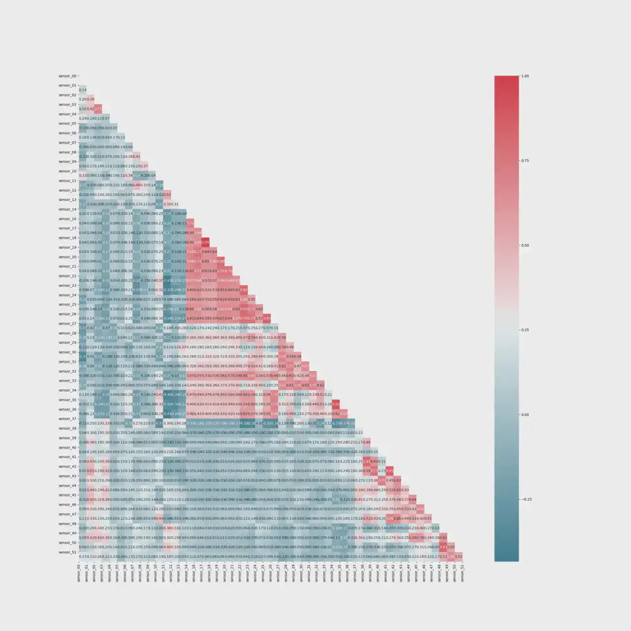
Spearman’s Correlation Heatmap
The heatmap indicates that we have few sensors that have a high positive correlation amongst one another. Additionally, sensor 48 - 51 have a moderate to high positive linear relationship with the output variable. The high correlation between our output variable and these sensors might be because of the sensors importance for the seven failures we have identified in our dataset. Our feature importance indicates that only 15 sensors have impact on the outcome. However, this might be because the fault within the machinery occurred in the “view” of these sensors and is not per se an indicator for, that we should remove information from other sensors, as they might be the once discovering a future breakdown. It is important to remember that we have only seen 7 breakdowns over the lifetime of the data which is unlikely to include all failures which can happen inside the water pump. Therefore, it is not necessarily a good idea to perform a feature extraction and remove features.
Random Forest
First we use a random forest for generating a prediction model as well as to generate feature importance. Additionally, we use Random Forest because it works great on unbalanced datasets. In this model, we keep all three classifications, and reassign them as 0 = Normal, 1 = Recovering, and 2 = Broken.
We then split our dataset into training, validation, and test, and rescale the dataset before fitting to our model
|
|
By using Random Forest, we can create a model with a 100% accuracy in both train, validation, and test. Now, this normally would call for concerns about whether the model is overfitting, however, we do get a perfect result in both our validation and test data. Additionally, based on the findings in the descriptive analysis, it could actually be true that we can reach this high accuracy, because each class differs significantly from one another. In the figure below our confusion matrix for train can be seen:

Confusion Matrix for Train
As our dataset contains few observations of type broken, our validation data do not have any observations of this value. We therefore “only” get a 2x2 matrix for normal and recovering when looking at validation:
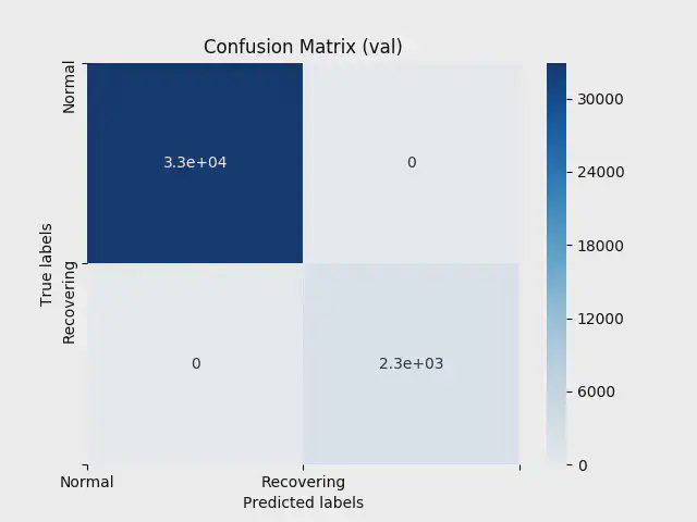
Finally, our test data shows the following:
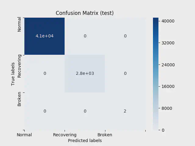
Confusion matrix for test
The Random Forest only indicates in which state our machinery is at now, and not in which direction it is heading towards. In other words it is good for saying if the machine is broken right now but not if it will break in the future. It does however, still create useful insight.
If we create a serial connected chain of models where the Random Forest model is the first it can be used to spot recovering and “warming up”. This can tell our prediction model when the machinery is recovering or “warming up”, as this data is irrelevant, and we can make sure to not predict in that time span, reducing the probability of false negative predictions.
To predict future probability for breakdown, we will use Long Short-Term Memory.
Long Short-Term Memory
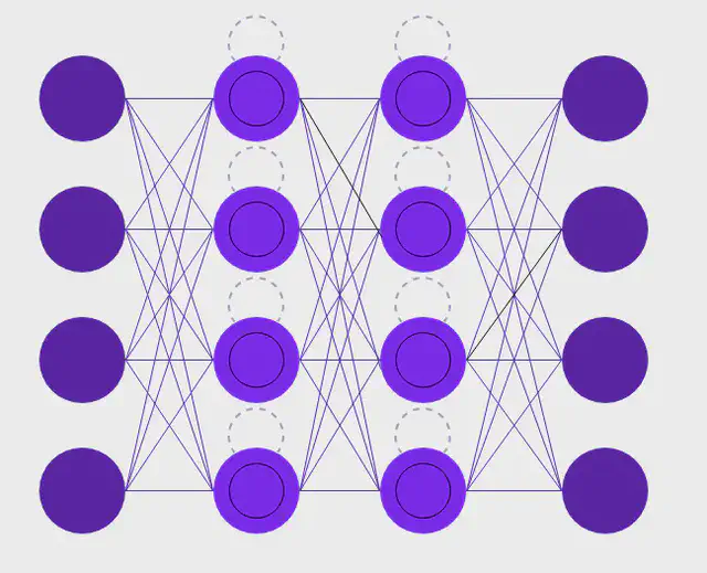
Long Short-Term Memory (LSTM) is a complex neural network with a memory cell, input, output, and forget (gates) (see figure below). The memory cell can store previous data in a specified amount, which can be used to help improve the prediction. By the help of a gate, it is possible to add or remove information to a cell. Each cell has three gates with the objective to protect, and control the cell.
The LSTM algorithm needs an input shape that is 3-dimensional. The three dimensions are:
- Batch size: the number of observations.
- Time steps: how many previous observations to remember.
- Features (input_dim): the number of different features that we use to predict the outcome. Before we reshape our dataset to 3D, we need to preprocess the data.
We drop all data of which the output variable is equal to “Recovering” and transform our output to binary values of which “Normal” = 1, and “Broken" = 0. To do that, we use LabelEncoder:
|
|
We split our dataset in to train, validation, and test, so we have 101,886 observations for our training session, 30,877 observations for validation, and 82,338 observations for testing. We rescale our data, and use PCA for dimensionality reduction.
Now is the time to reshape our data in to the required 3D. We wish our model to be able to store seven observations in its memory cell and use that for help in predicting the probability of machinery failure. When both train, test, and validation data is split, it is time to design our LSTM architecture which consists of an input layer, two LSTM-layers, and an output layer with one neuron, as our output value is binary:
|
|
We use earlystopper and checkpointer to reduce the probability of overfitting, and are now ready to train:
|
|
We get a train accuracy score of 99.99%, a validation accuracy of 99.99% and a test data that provides an accuracy score of 99.99%. When testing our model on the entire dataset we reach an accuracy score is 99.48% with a ROC AUC score of 96.59%.
This is great! However, we are actually not that interested in the classification, neither the confusion matrix below that shows us that we only predicts 5 out of 2 machinery failures correctly, or we have 2,779 false positives. We are interested in how well our model correctly predicts the probability of future breakdown. This means that we accept some false positives, as these works as a mark for a coming failure. Additionally, we might not predict the failure at the exact moment the machine fails. However, we would rather have some predictions prior to this happening, indicating that something is wrong.
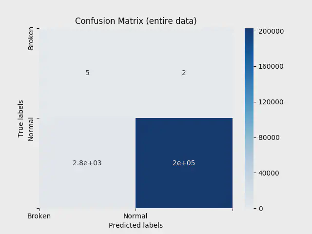
Confusion Matrix on Entire Data
It is important to be aware of what we are aiming to predict, and we are not interested in getting to know the machine fails, at the moment it fails - everyone working around the machine can see that. We are interested in getting warnings before that occurs, which is why the confusion matrix is, to some degree, irrelevant!. To determine whether we are satisfied with our model, we need further investigation - now is the time for predictions!
We know that we have a machinery failure the 12th of April 2018, at 09:55 pm. To see how well our model spots this failure prior to it happening, we run a simple probability test. When running the probability test, we can see that our model predicts a zero to no probability of machinery failure on the days before it happens. However, when we reach exactly 30 observations prior to the breakdown, we continually get warnings about a failure occurring with a very high probability (0.85% and increasing to 98%). Additionally, we can see the probability slowly increases from each observation until the failure, making a great prediction for machinery failure! The false positives in our model actually contributes with this probability being so strong that we can predict its occurence 30 observations before the failure! Finally, when the machine is running normal for a longer time, the probability of failure lies between 0-5%.
Just for fun, let us predict one more: We know that we have a failure the 8th of July 2018 at 11:00. When testing our models capability to detect this failure we get an increased probability of failure 38 observations prior to the failure, making it possible to take actions in time and prevent the breakdown to be of more severe.
Conclusion
Predictive maintenance can significantly improve your company’s OEE score by increasing the Availability and indirectly improving the Performance. Moreover, it can significantly reduce total production costs and increase delivery capabilities!
Even though our model do not predict all failures correctly at the exact time it occurs, it predicts a failure will occur prior to it happening (the false positives), giving us time to maintain the machinery and prevent a more severe breakdown. With this dataset, we are capable of predicting almost all failures prior to them happening, even though our confusion matrix indicates differently. We are capable of predicting a future breakdown 7 to 38 observations prior to the failure occurs!
// Maria Hvid, Machine Learning Engineer @ neurospace
References
Slack et al (2016) Operations Management (8th edition) Pearson